A cellular automaton is a system consisting of cells of numerical values on a grid, together with a rule that decides the behaviour of these cells. By applying the rule repeatedly on each cell in the grid while visualising the grid in some way or another, one often gets the effect of some evolving organism with complex and intricate behavior, even from relatively simple rules.

Cellular automata comes in many shapes, forms and dimensions. Perhaps the most famous cellular automaton is Conway's Game of Life (GOL). It consists of a two-dimensional grid where each cell contain a boolean value (dead or alive). The accompanying rule decides whether or not a cell should be dead or alive based on that cell's neighbouring cells. It states that a live cell dies of loneliness if there are less than 2 live cells around it. Similarly, it dies of overcrowding if more than three neighbouring cells are alive. In other words, a cell will only "survive" by having exactly 2 or 3 neighbouring cells that are alive. For a dead cell to become alive, it needs to have exactly 3 live neighbouring cells, otherwise it stays dead. An example of the GoL automaton can be seen below, iterating rapidly through several states.

Another famous cellular automaton variant is a one-dimensional one, called the Elementary Cellular Automaton (ECA). This is the one we will be implementing in this post.

Each state of this automaton is stored as a one-dimensional boolean array, and while GOL requires two dimensions to visualise its state, this automaton requires only a single line of values. Because of this, we can use two dimensions (rather than an animation) to visualise the whole state history of this automaton. As with GOL, the state of a cell in this automaton is either 0 or 1, but while a cell in GOL is updated based on its 8 neighbours, ECA has its cell updated based on its left neighbour, its right neighbour and itself!

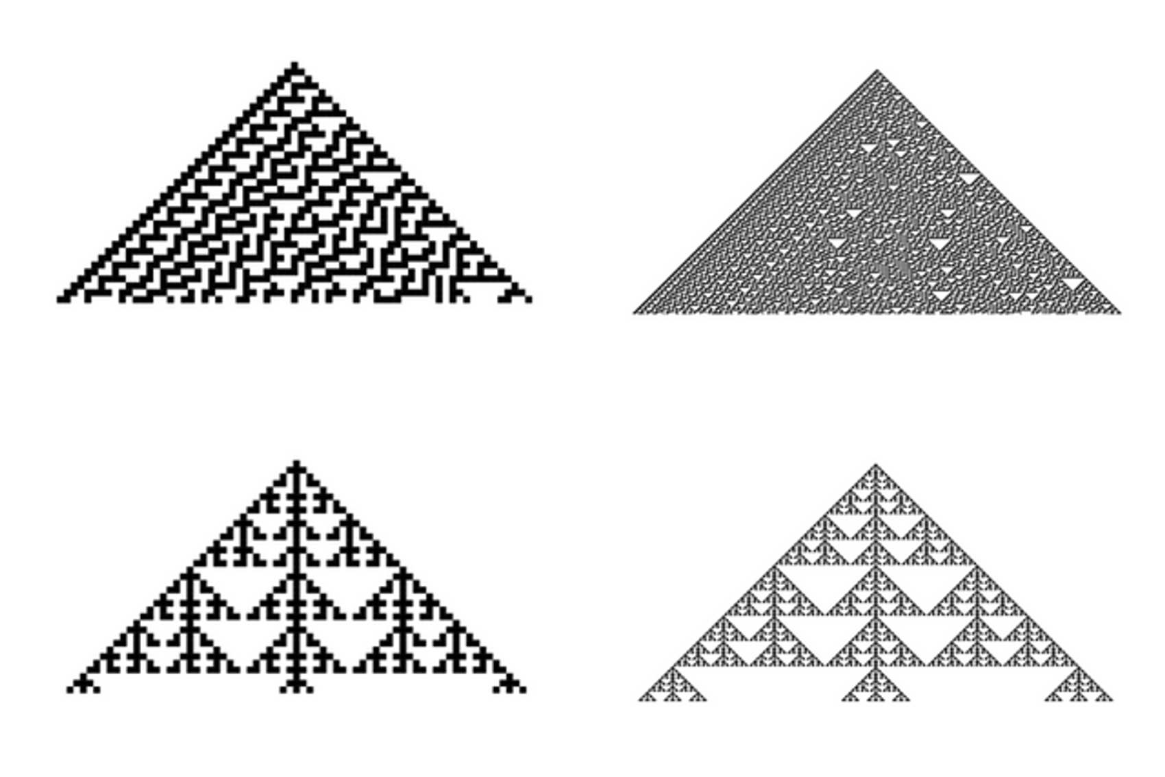
You can see examples of rules below, with the three top cells being the input of the rule, and the single bottom cell being the output, black being 1, white being 0. You also see the patterns each of them generates, with the initial condition being all 0's except a 1 in the middle cell.

You might wonder why the above rules have numbers attached to them. This is because each number between 0 and 255 directly corresponds to an ECA rule, and is thus used to name the rules. This subtle correspondence is shown below:

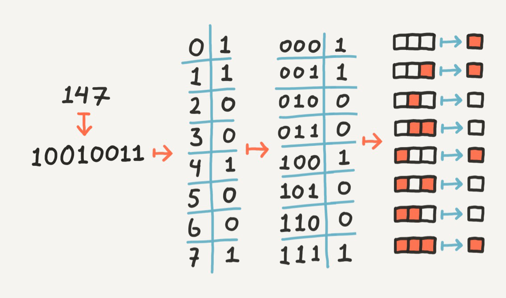
Any number in the interval from 0 through 255 can be represented in binary using only 8 digits (first arrow above). Furthermore, we can give each of these 8 digits an index based on their positioning (second arrow). These indices will naturally range between 0 and 7, which coincidentally are numbers that can be represented in binary using only 3 digits (third arrow). By interpreting these 3 digits as input, and the corresponding digit from our original number as output, we get the tertiary function we are looking for (fourth arrow).

Generating rules

Let's implement the above interpretation as a higher-order function get_rule that takes a number between 0 and 255 as its input and returns the ECA rule corresponding to that number.

We want it to work somewhat like this:

const rule30 = get_rule(30);
const output110 = rule30(1, 1, 0);

In the above example, running rule30(1,1,0) will combine the three binary values into a single number (110 = 6) and return the bit at that position (6) in the binary representation of 30. 30 is 00011110 in binary, so the function will return 0 (we do our counting from the right, and start counting from 0).

Knowing that the three binary input variables will be combined into one number, let's start by implementing such a combine function.

const combine = (b1, b2, b3) => (b1 << 2) + (b2 << 1) + (b3 << 0);

By left-shifting the arguments to their appropriate positions, then adding the three shifted numbers, we get the combination we were looking for.

The second important part of the get_rule function is to figure out what bit value is located at a certain position in a number. Let's therefore build the function get_bit(num, pos) that can return the bit value at a given position pos in a given number num. For instance, the number 141 is 10001101 in binary, so get_bit(2, 141) should return 1, while get_bit(5, 141) should return 0 .

get_bit(num,pos) can be implemented by first bitshifting our number pos positions to the right and then do a bitwise AND with the number 1.

const get_bit = (num, pos) => (num >> pos) & 1;

Now it just a matter of putting these two functions together:

const get_rule = (num) => (b1, b2, b3) => get_bit(num, combine(b1, b2, b3));

Cool! We now have a function that for each number between within our interval gives us a unique ECA rule that we can do whatever we want with. The next step is to visualise them in the browser.

Visualising rules

We will use a canvas element to visualise our automata in the browser. A canvas element can be created and added to the body of your html in the following way:

window.onload = function () {
  const canvas = document.createElement("canvas");
  canvas.width = 800;
  canvas.height = 800;

  document.body.appendChild(canvas);
};

In order to interact with our canvas, we need a context. A context is what lets us draw shapes and lines, give things colour, and generally move around on our canvas. It is provided for us through the getContext method on our canvas.

const context = canvas.getContext("2d");

The '2d' parameter refers to the context type we will be using in this example.

Next, we make a function that, given a context, an ECA rule and some info on the scale and number of our cells, draws the rule onto our canvas. The idea is to generate and draw the grid row by row; with the main part of the code looking something like this:

function draw_rule(ctx, rule, scale, width, height) {
  let row = initial_row(width);
  for (let i = 0; i < height; i++) {
    draw_row(ctx, row, scale);
    row = next_row(row, rule);
  }
}

We start off with some initial collection of cells as our current row. This row, like in the examples above, usually contains all 0s except for a 1 in the middle cell, but it can also contain a completely random string on 1s and 0s. We draw this row of cells, then calculate the next row of values based on our current row, using our rule. Then we simply repeat drawing and calculating new steps until we feel that our grid is tall enough.

The above code snippet requires us to implement 3 functions: initial_row, draw_row and next_row.

initial_row is a simple function. Make an array of 0s and change the element in the middle of the array to a 1.

function initial_row(length) {
  const initial_row = Array(length).fill(0);
  initial_row[Math.floor(length / 2)] = 1;

  return initial_row;
}

With our rule function readily available, the next_row function can be written as a oneliner. Each cell value in the new row is the product of our rule with the nearby cell values in the old row as input.

const next_row = (row, rule) =>
  row.map((_, i) => rule(row[i - 1], row[i], row[i + 1]));

Do you notice our cheat in the line above? Each cell in our new row needs input from three other cells, but the two cells at each edge of the row only gets input from two. For instance, next_row[0] tries to get an input value from row[-1]. This works because javascript returns undefined when attempting to access values at indices that don't exist in an array, and it so happens that (undefined >> [any number]) (from our combine function) always returns 0. This means that we in reality treat every value outside our grid as a 0.

I know, it's not pretty, but we are making something really pretty on the screen very soon, so we are excused.

Next up is our draw_row function; the one that actually does the drawing!

function draw_row(ctx, row, scale) {
  ctx.save();
  row.forEach((cell) => {
    ctx.fillStyle = cell === 1 ? "#000" : "#fff";
    ctx.fillRect(0, 0, scale, scale);
    ctx.translate(scale, 0);
  });
  ctx.restore();
  ctx.translate(0, scale);
}

This is where we are heavily depending on our context object, utilising no less than 5 different methods from it. Here is a quick look at each one, and how we use them.

• fillStyle specifies what you want to fill your shapes with. It can be a colour, like "#f55", but also a gradient or a pattern. We use it to distinguish between 0-cells and 1-cells.
• fillRect(x, y, w, h) draws a rectangle from point (x,y) with width w and height h, filled according to the fillStyle. Our rectangles are simple squares, but you might be surprised that they all are positioned in origo. This is because we use it in conjunction with translate.
• translate(x, y) lets you move the whole coordinate system around. This persists, so it works as a great alternative to keeping track of the different positions of items. For instance, instead of calculating the position of each individual cell in our grid, we can just draw a cell, move to the right, draw a new cell and so on.
• save() and restore() is used together with translate and other coordinate-transforming methods. We use them to save the current coordinate system at a certain point, so that we at a later point may return to it (using restore). In our case, we save our coordinate system before we start drawing a row and move to the right. Then, when we are done drawing the row and are all the way to the right, we restore, so we get back to our initial state. Finally we move down so that we are ready to start drawing the next row.

We now have all the parts needed for our draw_rule function. We will use this function on window.onload after having set up the canvas. We also define the parameters we need.

window.onload = function () {
  const width = 1000; // Width of the canvas
  const height = 500; // Height of the canvas

  const cells_across = 200; // Number of cells horizontally in the grid
  const cell_scale = width / cells_across; // Size of each cell
  const cells_down = height / cell_scale; // Number of cells vertically in the grid

  const rule = get_rule(30); // The rule to display

  const canvas = document.createElement("canvas");
  canvas.width = width;
  canvas.height = height;

  document.body.appendChild(canvas);

  const context = canvas.getContext("2d");
  draw_rule(context, rule, cell_scale, cells_across, cells_down);
};

We extract the canvas dimensions as individual variables together with the number of cells horizontally. Then, we calculate the cell_scale and 'cells_down' so that the grid fills the whole canvas while keeping cells square. This way, we can now easily change the "resolution" of our grid while still keeping it within the bounds of the canvas.

...and that's it! The full code example is available on github and as a codepen:

See the Pen oNgZKqV by Kjetil Golid (@kgolid) on CodePen.

Onward from here

Having this setup now lets you explore all the 256 different rules one by one, either by iterating through each one by changing the code, or by letting the rule number be random at every page load. Either way, it is a great feeling to explore these unpredictable results within your own controlled environment.

Another thing to explore is letting the initial cell state of our automata be random rather than our static "only 0s, but a single 1" state. This will yield even more unpredictable results. Such a variant of our initial_row can be written like this:

function random_initial_row(width) {
  return Array.from(Array(width), (_) => Math.floor(Math.random() * 2));
}

You can see below how big of an effect this change in the initial row has on the output.

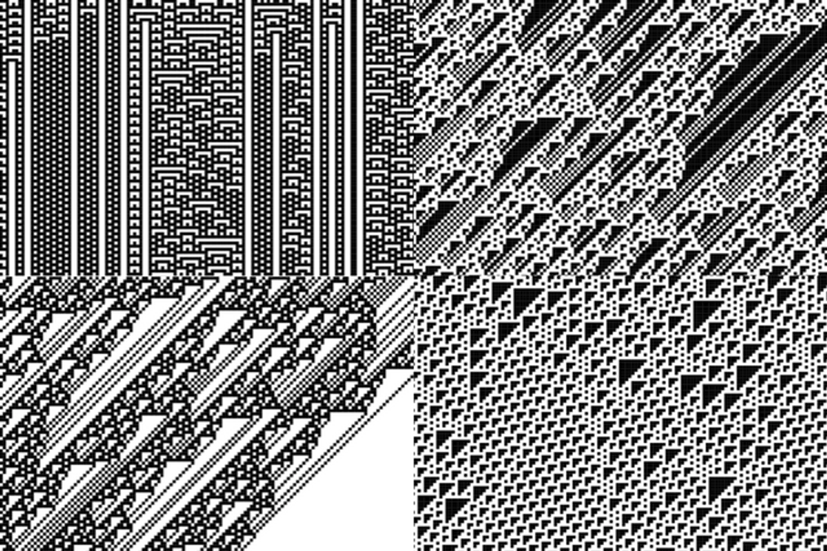
This is only one of the things you can change though! Why limit ourselves to two states? (Going from 2 to 3 states actually increases the number of rules from 256 to 7 625 597 484 987!) Why limit ourselves to squares? Why only 2 dimensions? Why only one rule at a time?

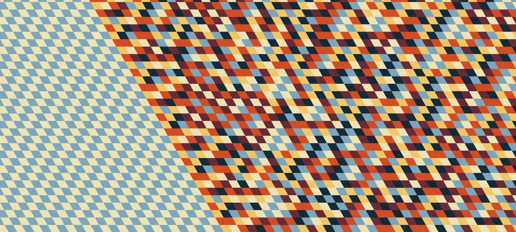
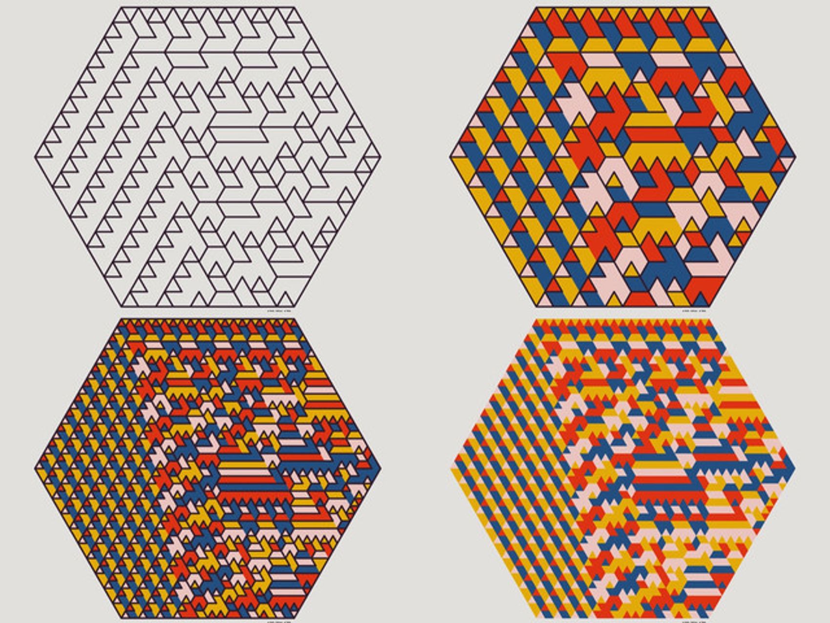
Below are some examples of ECA-based visualisations, but with an alternative draw_rule function, drawing lines in an isometric pattern rather than squares, then filling areas defined by those lines with colours. You can even choose to not display the separating lines at all, only showing the colours.

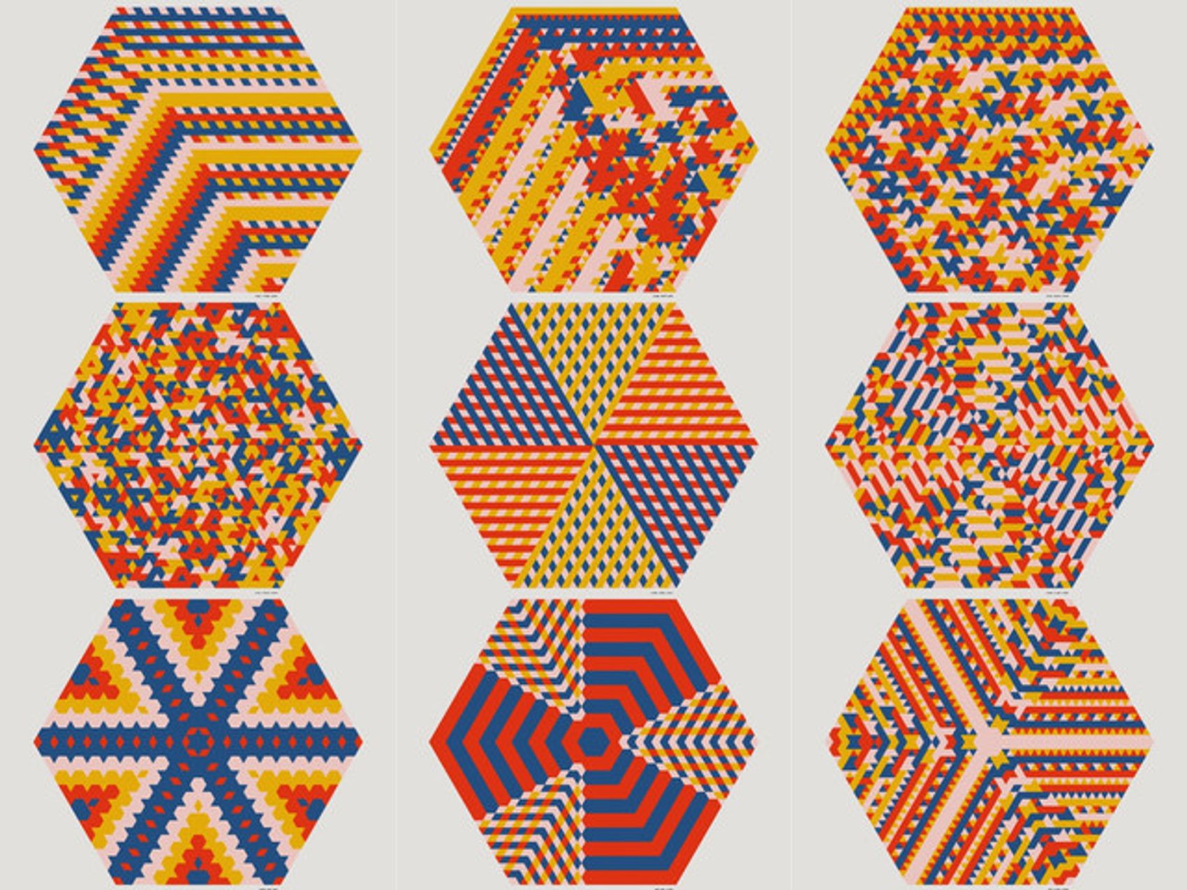
Taking it even further, one can start introducing symmetries, both rotational (middle row) and reflectional (bottom row).

If you find the above visuals interesting, feel free to check out this interactive playground, or even better, start from the code we've built here and try coming up with your very own cellular automata!

Good luck!