In the previous article we considered how noise reduction filters may be useful in practical applications. In this article we walk through the mathematical and technical aspects of implementing the noise reduction filters used there. We conclude with final remarks comparing our regularization operators to the broader class of moving averages. The reader is assumed to be conversant in elementary calculus.
Mathematical definition
In this section we build up to the mathematical definition of our discrete mollifier transforms. Considerations of implementation are found in the appropriate sections below.
The continuous case
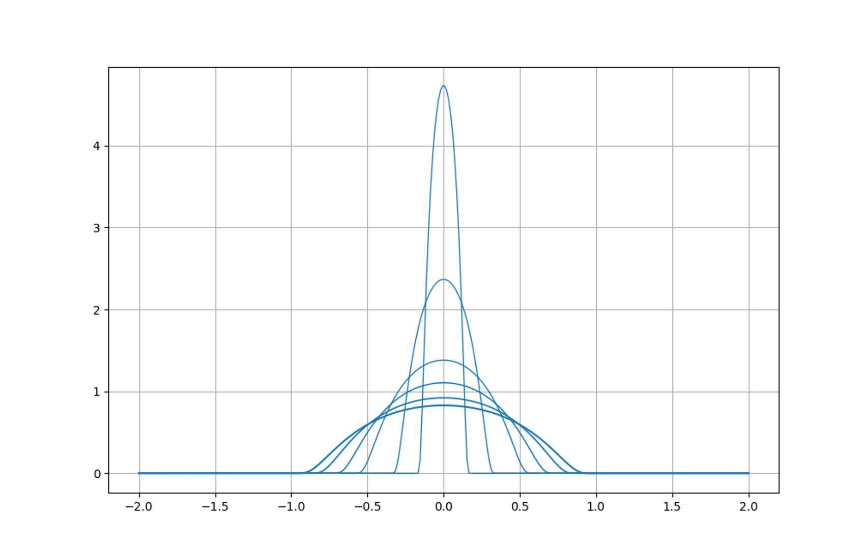
Pulling a rabbit out of the hat, consider the standard mollifier with parameter epsilon:

the constant A > 0 being chosen so that

To be particular,

The standard mollifiers are smooth (infinitely differentiable) functions vanishing outside the neighbourhood of the origin with radius epsilon.
The insight is that convolution against the standard mollifiers produces smooth functions, even if the original function undergoing the convolution is highly irregular. To be precise, introduce the integral operator sending a function to its convolution against the standard mollifiers:

We call this the mollification of u with parameter epsilon. The convolution is well-defined whenever u is locally integrable in the Lebesgue sense, in which case its mollification is in fact a smooth function. We have thus obtained the smoothing operator in the continuous case:

It is from the good convergence properties of the mollifications back to the original function, as epsilon tends to zero, that the procedure gains its attractiveness. We will not delve into further details on that matter here, preferring instead to turn our attention to the discretization of the mollification operators themselves.
The discrete case
To discretize the mollification operators, we approximate the integrals defining the mollification of a locally integrable function u by means of the trapezoidal rule. Other schemes for numerical quadrature may be applied, but the trapezoidal method reduces in the final analysis down to a particularly nice convolutional form suitable for efficient implementation on a computer, and obtains satisfactory error bounds.
Construe now u as being sampled at n equidistant points, indexed from 0 to n-1, and take epsilon to be k≥1 times the mesh size. Abusing notation ever so slightly, the integral we wish to approximate at index j is thus

Sparing the reader the inevitable juggling of indicies, the discrete mollification of u at index j works out to be

at least for indicies j satisfying 0 ≤ j-k < j+k ≤ n-1, that is, for k ≤ j ≤ n-k-1. It is this form we next seek to implement.
Implementation
We consider the naive implementation of the discrete mollification in Python. It is a simple exercise to port this snippet into any sensible programming language. Readers concerned with efficiency may consult the following subsection and optimize as they see fit.
Translating the discrete mollification operator above into Python directly produces:
import numpy as np
_NORMALIZATION_CONSTANT = 2.2522836210436354
def _mollifier(t: float) -> float:
"""Standard mollifier corresponding to epsilon = 1."""
return _NORMALIZATION_CONSTANT*np.exp(1.0/(t*t - 1.0)) if abs(t) < 1.0 else 0.0
def mollify(u: np.ndarray, k: int) -> np.ndarray:
"""Returns the discrete mollification of the given signal with window size `k`."""
if not isinstance(k, int):
raise TypeError(f"Window size must be an integer: {k=}")
if k < 1:
raise ValueError(f"Window size must be at least 1: {k=}")
if len(u.shape) > 1:
raise ValueError(f"Input signal must be one-dimensional: {u}")
n = u.size
Mu = np.copy(u)
for j in range(k, n - k):
Mu[j] = sum(_mollifier(i/k)*u[j - i] for i in range(1 - k, k))/k
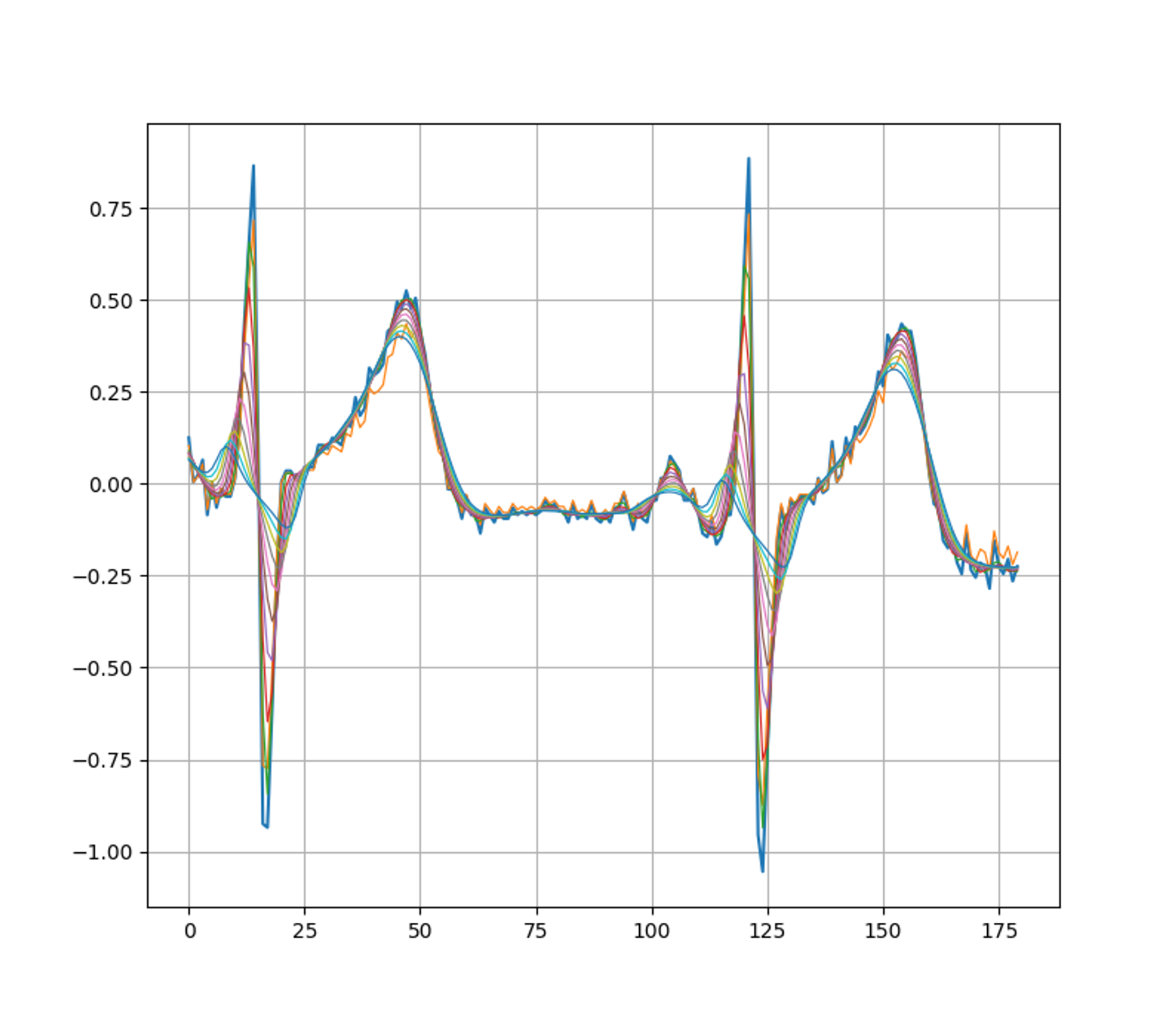
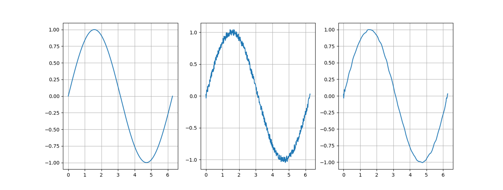
return MuThe effectiveness of the discrete smoothing operator defined above may be witnessed in the following figure.
Optimizations
Considering the convolutional form of the discrete mollification operators, the computational efficiency may be improved by precomputing the weights for various k and performing the convolution in a more optimized fashion, say through scipy.signal.fftconvolve. We undertake no such endevaour here.
Correcting the tails
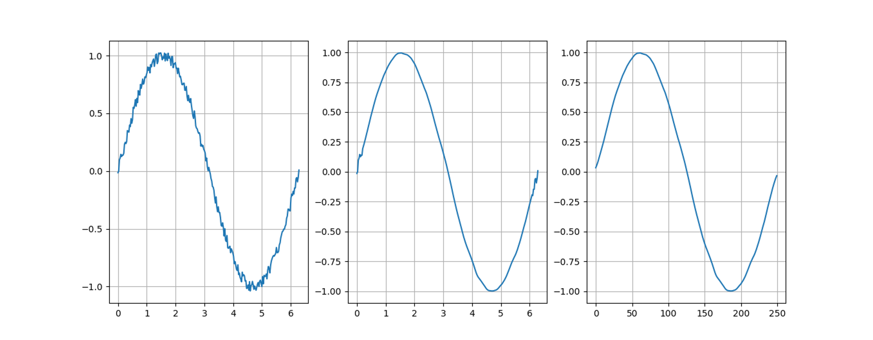
The attentive reader may have noticed that the first and last k sample points of the original signal are left unaltered by our implementation, producing noisy artifacts at the tails of our filtered signal. This is undesirable and easy to fix.
Remembering that the discrete mollification is only defined for indicies j satisfying k ≤ j ≤ (n-1)-k, we may simply pad our signal at both ends so as to achieve these inequalities for the portion of the padded signal corresponding to the original signal. In code:
import numpy as np

_NORMALIZATION_CONSTANT = 2.2522836210436354

def _mollifier(t: float) -> float:
    """Standard mollifier corresponding to epsilon = 1."""
    return _NORMALIZATION_CONSTANT*np.exp(1.0/(t*t - 1.0)) if abs(t) < 1.0 else 0.0

def _mollify(u: np.ndarray, k: int) -> np.ndarray:
    """Returns the discrete mollification of the given signal with window size `k`."""
    if not isinstance(k, int):
        raise TypeError(f"Window size must be an integer: {k=}")
    if k < 1:
        raise ValueError(f"Window size must be at least 1: {k=}")
    if len(u.shape) > 1:
        raise ValueError(f"Input signal must be one-dimensional: {u}")
    n = u.size
    Mu = np.copy(u)
    for j in range(k, n - k):
        Mu[j] = sum(_mollifier(i/k)*u[j - i] for i in range(1 - k, k))/k
    return Mu

def mollify(u: np.ndarray, k: int) -> np.ndarray:
    """Mollification filter with corrected tails."""
    n = u.size
    padded = np.zeros(n + 2*k)
    padded[:k] = u[0]
    padded[k:k + n] = u
    padded[k + n:] = u[-1]
    mollified = _mollify(padded, k)
    return mollified[k:n + k]
Here is the result:
Comparison with the class of moving averages
We now conclude with a brief comparison of our discrete mollifiers with the broader class of moving averages. A moving average is a convolutional operator of the form

with the weights summing to unity:

Even though our discrete mollifiers are not strictly of the moving average type, they are so asymptotically. Indeed, one may show the estimate

for some constant M≥0 independent of k, proving

Summary
In this article we have undertaken the construction, analysis, and implementation of a family of discrete smoothing operators. Furthermore, the convolutional form of these operators paves the way for efficient implementation in any programming language, making noise reduction filters broadly available. We also related the discrete mollifiers defined here to the broader class of moving averages, discovering their asymptotic membership to this class.